2.2. Mathematical Considerations
ARKODE solves ODE initial value problems (IVP) in \(\mathbb{R}^N\) posed in the form
Here, \(t\) is the independent variable (e.g. time), and the dependent variables are given by \(y \in \mathbb{R}^N\), where we use the notation \(\dot{y}\) to denote \(\mathrm dy/\mathrm dt\).
For each value of \(t\), \(M(t)\) is a user-specified linear operator from \(\mathbb{R}^N \to \mathbb{R}^N\). This operator is assumed to be nonsingular and independent of \(y\). For standard systems of ordinary differential equations and for problems arising from the spatial semi-discretization of partial differential equations using finite difference, finite volume, or spectral finite element methods, \(M\) is typically the identity matrix, \(I\). For PDEs using standard finite-element spatial semi-discretizations, \(M\) is typically a well-conditioned mass matrix that is fixed throughout a simulation (or at least fixed between spatial rediscretization events).
The ODE right-hand side is given by the function \(f(t,y)\) – in general we make no assumption that the problem (2.5) is autonomous (i.e., \(f=f(y)\)) or linear (\(f=Ay\)). In general, the time integration methods within ARKODE support additive splittings of this right-hand side function, as described in the subsections that follow. Through these splittings, the time-stepping methods currently supplied with ARKODE are designed to solve stiff, nonstiff, mixed stiff/nonstiff, and multirate problems. As per Ascher and Petzold [14], a problem is “stiff” if the stepsize needed to maintain stability of the forward Euler method is much smaller than that required to represent the solution accurately.
In the sub-sections that follow, we elaborate on the numerical methods utilized in ARKODE. We first discuss the “single-step” nature of the ARKODE infrastructure, including its usage modes and approaches for interpolated solution output. We then discuss the current suite of time-stepping modules supplied with ARKODE, including
ARKStep for additive Runge–Kutta methods
ERKStep that is optimized for explicit Runge–Kutta methods
ForcingStep for a forcing method
LSRKStep that supports low-storage Runge–Kutta methods
SplittingStep for operator splitting methods
SPRKStep for symplectic partitioned Runge–Kutta methods
We then discuss the adaptive temporal error controllers shared by the time-stepping modules, including discussion of our choice of norms for measuring errors within various components of the solver.
We then discuss the nonlinear and linear solver strategies used by ARKODE for solving implicit algebraic systems that arise in computing each stage and/or step: nonlinear solvers, linear solvers, preconditioners, error control within iterative nonlinear and linear solvers, algorithms for initial predictors for implicit stage solutions, and approaches for handling non-identity mass-matrices.
We conclude with a section describing ARKODE’s rootfinding capabilities, that may be used to stop integration of a problem prematurely based on traversal of roots in user-specified functions.
2.2.1. Adaptive single-step methods
The ARKODE infrastructure is designed to support single-step, IVP integration methods, i.e.
where \(y_{n-1}\) is an approximation to the solution \(y(t_{n-1})\), \(y_{n}\) is an approximation to the solution \(y(t_n)\), \(t_n = t_{n-1} + h_n\), and the approximation method is represented by the function \(\varphi\).
The choice of step size \(h_n\) is determined by the time-stepping method (based on user-provided inputs, typically accuracy requirements). However, users may place minimum/maximum bounds on \(h_n\) if desired.
ARKODE may be run in a variety of “modes”:
NORMAL – The solver will take internal steps until it has just overtaken a user-specified output time, \(t_\text{out}\), in the direction of integration, i.e. \(t_{n-1} < t_\text{out} \le t_{n}\) for forward integration, or \(t_{n} \le t_\text{out} < t_{n-1}\) for backward integration. It will then compute an approximation to the solution \(y(t_\text{out})\) by interpolation (using one of the dense output routines described in the section §2.2.2).
ONE-STEP – The solver will only take a single internal step \(y_{n-1} \to y_{n}\) and then return control back to the calling program. If this step will overtake \(t_\text{out}\) then the solver will again return an interpolated result; otherwise it will return a copy of the internal solution \(y_{n}\).
NORMAL-TSTOP – The solver will take internal steps until the next step will overtake \(t_\text{out}\). It will then limit this next step so that \(t_n = t_{n-1} + h_n = t_\text{out}\), and once the step completes it will return a copy of the internal solution \(y_{n}\).
ONE-STEP-TSTOP – The solver will check whether the next step will overtake \(t_\text{out}\) – if not then this mode is identical to “one-step” above; otherwise it will limit this next step so that \(t_n = t_{n-1} + h_n = t_\text{out}\). In either case, once the step completes it will return a copy of the internal solution \(y_{n}\).
We note that interpolated solutions may be slightly less accurate than the internal solutions produced by the solver. Hence, to ensure that the returned value has full method accuracy one of the “tstop” modes may be used.
2.2.2. Interpolation
As mentioned above, the ARKODE supports interpolation of solutions \(y(t_\text{out})\) and derivatives \(y^{(d)}(t_\text{out})\), where \(t_\text{out}\) occurs within a completed time step from \(t_{n-1} \to t_n\). Additionally, this module supports extrapolation of solutions and derivatives for \(t\) outside this interval (e.g. to construct predictors for iterative nonlinear and linear solvers). To this end, ARKODE currently supports construction of polynomial interpolants \(p_q(t)\) of polynomial degree up to \(q=5\), although users may select interpolants of lower degree.
ARKODE provides two complementary interpolation approaches: “Hermite” and “Lagrange”. The former approach has been included with ARKODE since its inception, and is more suitable for non-stiff problems; the latter is a more recent approach that is designed to provide increased accuracy when integrating stiff problems. Both are described in detail below.
2.2.2.1. Hermite interpolation module
For non-stiff problems, polynomial interpolants of Hermite form are provided. Rewriting the IVP (2.5) in standard form,
we typically construct temporal interpolants using the data \(\left\{ y_{n-1}, \hat{f}_{n-1}, y_{n}, \hat{f}_{n} \right\}\), where here we use the simplified notation \(\hat{f}_{k}\) to denote \(\hat{f}(t_k,y_k)\). Defining a normalized “time” variable, \(\tau\), for the most-recently-computed solution interval \(t_{n-1} \to t_{n}\) as
we then construct the interpolants \(p_q(t)\) as follows:
\(q=0\): constant interpolant
\[p_0(\tau) = \frac{y_{n-1} + y_{n}}{2}.\]\(q=1\): linear Lagrange interpolant
\[p_1(\tau) = -\tau\, y_{n-1} + (1+\tau)\, y_{n}.\]\(q=2\): quadratic Hermite interpolant
\[p_2(\tau) = \tau^2\,y_{n-1} + (1-\tau^2)\,y_{n} + h_n(\tau+\tau^2)\,\hat{f}_{n}.\]\(q=3\): cubic Hermite interpolant
\[p_3(\tau) = (3\tau^2 + 2\tau^3)\,y_{n-1} + (1-3\tau^2-2\tau^3)\,y_{n} + h_n(\tau^2+\tau^3)\,\hat{f}_{n-1} + h_n(\tau+2\tau^2+\tau^3)\,\hat{f}_{n}.\]\(q=4\): quartic Hermite interpolant
\[\begin{split}p_4(\tau) &= (-6\tau^2 - 16\tau^3 - 9\tau^4)\,y_{n-1} + (1 + 6\tau^2 + 16\tau^3 + 9\tau^4)\,y_{n} + \frac{h_n}{4}(-5\tau^2 - 14\tau^3 - 9\tau^4)\,\hat{f}_{n-1} \\ &+ h_n(\tau + 2\tau^2 + \tau^3)\,\hat{f}_{n} + \frac{27 h_n}{4}(-\tau^4 - 2\tau^3 - \tau^2)\,\hat{f}_a,\end{split}\]where \(\hat{f}_a=\hat{f}\left(t_{n} - \dfrac{h_n}{3},p_3\left(-\dfrac13\right)\right)\). We point out that interpolation at this degree requires an additional evaluation of the full right-hand side function \(\hat{f}(t,y)\), thereby increasing its cost in comparison with \(p_3(t)\).
\(q=5\): quintic Hermite interpolant
\[\begin{split}p_5(\tau) &= (54\tau^5 + 135\tau^4 + 110\tau^3 + 30\tau^2)\,y_{n-1} + (1 - 54\tau^5 - 135\tau^4 - 110\tau^3 - 30\tau^2)\,y_{n} \\ &+ \frac{h_n}{4}(27\tau^5 + 63\tau^4 + 49\tau^3 + 13\tau^2)\,\hat{f}_{n-1} + \frac{h_n}{4}(27\tau^5 + 72\tau^4 + 67\tau^3 + 26\tau^2 + \tau)\,\hat{f}_n \\ &+ \frac{h_n}{4}(81\tau^5 + 189\tau^4 + 135\tau^3 + 27\tau^2)\,\hat{f}_a + \frac{h_n}{4}(81\tau^5 + 216\tau^4 + 189\tau^3 + 54\tau^2)\,\hat{f}_b,\end{split}\]where \(\hat{f}_a=\hat{f}\left(t_{n} - \dfrac{h_n}{3},p_4\left(-\dfrac13\right)\right)\) and \(\hat{f}_b=\hat{f}\left(t_{n} - \dfrac{2h_n}{3},p_4\left(-\dfrac23\right)\right)\). We point out that interpolation at this degree requires four additional evaluations of the full right-hand side function \(\hat{f}(t,y)\), thereby significantly increasing its cost over \(p_4(t)\).
We note that although interpolants of order \(q > 5\) are possible, these are not currently implemented due to their increased computing and storage costs.
2.2.2.2. Lagrange interpolation module
For stiff problems where \(\hat{f}\) may have large Lipschitz constant, polynomial interpolants of Lagrange form are provided. These interpolants are constructed using the data \(\left\{ y_{n}, y_{n-1}, \ldots, y_{n-\nu} \right\}\) where \(0\le\nu\le5\). These polynomials have the form
Since we assume that the solutions \(y_{n-j}\) have length much larger than \(\nu\le5\) in ARKODE-based simulations, we evaluate \(p\) at any desired \(t\in\mathbb{R}\) by first evaluating the Lagrange polynomial basis functions at the input value for \(t\), and then performing a simple linear combination of the vectors \(\{y_k\}_{k=0}^{\nu}\). Derivatives \(p^{(d)}(t)\) may be evaluated similarly as
however since the algorithmic complexity involved in evaluating derivatives of the Lagrange basis functions increases dramatically as the derivative order grows, our Lagrange interpolation module currently only provides derivatives up to \(d=3\).
We note that when using this interpolation module, during the first \((\nu-1)\) steps of integration we do not have sufficient solution history to construct the full \(\nu\)-degree interpolant. Therefore during these initial steps, we construct the highest-degree interpolants that are currently available at the moment, achieving the full \(\nu\)-degree interpolant once these initial steps have completed.
2.2.3. ARKStep – Additive Runge–Kutta methods
The ARKStep time-stepping module in ARKODE is designed for IVPs of the form
i.e. the right-hand side function is additively split into two components:
\(f^E(t,y)\) contains the “nonstiff” components of the system (this will be integrated using an explicit method);
\(f^I(t,y)\) contains the “stiff” components of the system (this will be integrated using an implicit method);
and the left-hand side may include a nonsingular, possibly time-dependent, matrix \(M(t)\).
In solving the IVP (2.6), we first consider the corresponding problem in standard form,
where \(\hat{f}^E(t,y) = M(t)^{-1}\,f^E(t,y)\) and \(\hat{f}^I(t,y) = M(t)^{-1}\,f^I(t,y)\). ARKStep then utilizes variable-step, embedded, additive Runge–Kutta methods (ARK), corresponding to algorithms of the form
Here \(\tilde{y}_n\) are embedded solutions that approximate \(y(t_n)\) and are used for error estimation; these typically have slightly lower accuracy than the computed solutions \(y_n\). The internal stage times are abbreviated using the notation \(t^E_{n,j} = t_{n-1} + c^E_j h_n\) and \(t^I_{n,j} = t_{n-1} + c^I_j h_n\). The ARK method is primarily defined through the coefficients \(A^E \in \mathbb{R}^{s\times s}\), \(A^I \in \mathbb{R}^{s\times s}\), \(b^E \in \mathbb{R}^{s}\), \(b^I \in \mathbb{R}^{s}\), \(c^E \in \mathbb{R}^{s}\) and \(c^I \in \mathbb{R}^{s}\), that correspond with the explicit and implicit Butcher tables. Additional coefficients \(\tilde{b}^E \in \mathbb{R}^{s}\) and \(\tilde{b}^I \in \mathbb{R}^{s}\) are used to construct the embedding \(\tilde{y}_n\). We note that ARKStep currently enforces the constraint that the explicit and implicit methods in an ARK pair must share the same number of stages, \(s\). We note that except when the problem has a time-independent mass matrix \(M\), ARKStep allows the possibility for different explicit and implicit abscissae, i.e. \(c^E\) need not equal \(c^I\).
The user of ARKStep must choose appropriately between one of three classes of methods: ImEx, explicit, and implicit. All of the built-in Butcher tables encoding the coefficients \(c^E\), \(c^I\), \(A^E\), \(A^I\), \(b^E\), \(b^I\), \(\tilde{b}^E\) and \(\tilde{b}^I\) are further described in the section §2.8.
For mixed stiff/nonstiff problems, a user should provide both of the functions \(f^E\) and \(f^I\) that define the IVP system. For such problems, ARKStep currently implements the ARK methods proposed in [67, 93, 96], allowing for methods having order of accuracy \(q = \{2,3,4,5\}\) and embeddings with orders \(p = \{1,2,3,4\}\); the tables for these methods are given in section §2.8.3. Additionally, user-defined ARK tables are supported.
For nonstiff problems, a user may specify that \(f^I = 0\), i.e. the equation (2.6) reduces to the non-split IVP
In this scenario, the coefficients \(A^I=0\), \(c^I=0\), \(b^I=0\) and \(\tilde{b}^I=0\) in (2.8), and the ARK methods reduce to classical explicit Runge–Kutta methods (ERK). For these classes of methods, ARKODE provides coefficients with orders of accuracy \(q = \{2,3,4,5,6,7,8,9\}\), with embeddings of orders \(p = \{1,2,3,4,5,6,7,8\}\); the tables for these methods are given in section §2.8.1. As with ARK methods, user-defined ERK tables are supported.
Alternately, for stiff problems the user may specify that \(f^E = 0\), so the equation (2.6) reduces to the non-split IVP
Similarly to ERK methods, in this scenario the coefficients \(A^E=0\), \(c^E=0\), \(b^E=0\) and \(\tilde{b}^E=0\) in (2.8), and the ARK methods reduce to classical diagonally-implicit Runge–Kutta methods (DIRK). For these classes of methods, ARKODE provides tables with orders of accuracy \(q = \{2,3,4,5\}\), with embeddings of orders \(p = \{1,2,3,4\}\); the tables for these methods are given in section §2.8.2. Again, user-defined DIRK tables are supported.
2.2.4. ERKStep – Explicit Runge–Kutta methods
The ERKStep time-stepping module in ARKODE is designed for IVP of the form
i.e., unlike the more general problem form (2.6), ERKStep requires that problems have an identity mass matrix (i.e., \(M(t)=I\)) and that the right-hand side function is not split into separate components.
For such problems, ERKStep provides variable-step, embedded, explicit Runge–Kutta methods (ERK), corresponding to algorithms of the form
where the variables have the same meanings as in the previous section.
Clearly, the problem (2.11) is fully encapsulated in the more general problem (2.9), and the algorithm (2.12) is similarly encapsulated in the more general algorithm (2.8). While it therefore follows that ARKStep can be used to solve every problem solvable by ERKStep, using the same set of methods, we include ERKStep as a distinct time-stepping module since this simplified form admits a more efficient and memory-friendly implementation than the more general form (2.11).
2.2.5. ForcingStep – Forcing method
The ForcingStep time-stepping module in ARKODE is designed for IVPs of the form
with two additive partitions. One step of the forcing method implemented in ForcingStep is given by
Like a Lie–Trotter method from SplittingStep, the partitions are evolved through a sequence of inner IVPs which can be solved with an arbitrary integrator or exact solution procedure. However, the IVP for partition two includes a “forcing” or “tendency” term \(f_1^*\) to strengthen the coupling. This coupling leads to a first order method provided \(v_1\) and \(v_2\) are integrated to at least first order accuracy. Currently, a fixed time step must be specified for the overall ForcingStep integrator, but partition integrators are free to use adaptive time steps.
2.2.6. LSRKStep – Low-Storage Runge–Kutta methods
The LSRKStep time-stepping module in ARKODE supports a variety of so-called “low-storage” Runge–Kutta (LSRK) methods, [60, 98, 109, 155]. This category includes traditional explicit fixed-step and low-storage Runge–Kutta methods, adaptive low-storage Runge–Kutta methods, and others. These are characterized by coefficient tables that have an exploitable structure, such that their implementation does not require that all stages be stored simultaneously. At present, this module supports explicit, adaptive “super-time-stepping” (STS) and “strong-stability-preserving” (SSP) methods.
The LSRK time-stepping module in ARKODE currently supports IVP of the form (2.11), i.e., unlike the more general problem form (2.6), LSRKStep requires that problems have an identity mass matrix (i.e., \(M(t)=I\)) and that the right-hand side function is not split into separate components.
LSRKStep currently supports two families of second-order, explicit, and temporally adaptive STS methods: Runge–Kutta–Chebyshev (RKC), [155] and Runge–Kutta–Legendre (RKL), [109]. These methods have the form
The corresponding coefficients can be found in [155] and [109], respectively.
LSRK methods of STS type are designed for stiff problems characterized by having Jacobians with eigenvalues that have large real and small imaginary parts. While those problems are traditionally treated using implicit methods, STS methods are explicit. To achieve stability for these stiff problems, STS methods use more stages than conventional Runge-Kutta methods to extend the stability region along the negative real axis. The extent of this stability region is proportional to the square of the number of stages used.
LSRK methods of the SSP type are designed to preserve the so-called “strong-stability” properties of advection-type equations. For details, see [98]. The SSPRK methods in ARKODE use the following Shu–Osher representation [133] of explicit Runge–Kutta methods:
The coefficients of the Shu–Osher representation are not uniquely determined by the Butcher table [142]. In particular, the methods SSP(s,2), SSP(s,3), and SSP(10,4) implemented herein and presented in [98] have “almost” all zero coefficients appearing in \(\alpha_{i,i-1}\) and \(\beta_{i,i-1}\). This feature facilitates their implementation in a low-storage manner. The corresponding coefficients and embedding weights can be found in [98] and [60], respectively.
2.2.7. MRIStep – Multirate infinitesimal step methods
The MRIStep time-stepping module in ARKODE is designed for IVPs of the form
i.e., the right-hand side function is additively split into three components:
\(f^E(t,y)\) contains the “slow-nonstiff” components of the system (this will be integrated using an explicit method and a large time step \(h^S_n\)),
\(f^I(t,y)\) contains the “slow-stiff” components of the system (this will be integrated using an implicit method and a large time step \(h^S_n\)), and
\(f^F(t,y)\) contains the “fast” components of the system (this will be integrated using a possibly different method than the slow time scale and a small time step \(h^F_n \ll h^S_n\)).
As with ERKStep, MRIStep currently requires that problems be posed with an identity mass matrix, \(M(t)=I\). The slow time scale may consist of only nonstiff terms (\(f^I \equiv 0\)), only stiff terms (\(f^E \equiv 0\)), or both nonstiff and stiff terms.
For cases with only a single slow right-hand side function (i.e., \(f^E \equiv 0\) or \(f^I \equiv 0\)), MRIStep provides multirate infinitesimal step (MIS) [126, 127, 128], first through fourth order multirate infinitesimal GARK (MRI-GARK) [123], and second through fifth order multirate exponential Runge–Kutta (MERK) [106] methods. For problems with an additively split slow right-hand side, MRIStep provides first through fourth order implicit-explicit MRI-GARK (IMEX-MRI-GARK) [39] and second through fourth order implicit-explicit multirate infinitesimal stage-restart (IMEX-MRI-SR) [62] methods. For a complete list of the methods available in MRIStep see §2.4.11.3.2. Additionally, users may supply their own method by defining and attaching a coupling table, see §2.4.11.3 for more information.
Generally, the slow (outer) method for each family derives from a single-rate method: MIS and MRI-GARK methods derive from explicit or diagonally-implicit Runge–Kutta methods, MERK methods derive from exponential Runge–Kutta methods, while IMEX-MRI-GARK and IMEX-MRI-SR methods derive from additive Runge–Kutta methods. In each case, the “infinitesimal” nature of the multirate methods derives from the fact that slow stages are computed by solving a set of auxiliary ODEs with a fast (inner) time integration method. Generally speaking, an \(s\)-stage method from of each family adheres to the following algorithm for a single step:
Set \(z_1 = y_{n-1}\).
For \(i = 2,\ldots,s\), compute the stage solutions, \(z_i\), by evolving the fast IVP
(2.16)\[{v}_i'(t) = f^F(t, v_i) + r_i(t) \quad\text{for}\quad t \in [t_{0,i},t_{F,i}] \quad\text{with}\quad v_i(t_{0,i}) = v_{0,i}\]and setting \(z_i = v(t_{F,i})\), and/or performing a standard explicit, diagonally-implicit, or additive Runge–Kutta stage update,
(2.17)\[z_i - \theta_{i,i} h^S_n f^I(t_{n,i}^S, z_i) = a_i.\]where \(t_{n,j}^S = t_{n-1} + h^S_n c^S_j\).
Set \(y_{n} = z_{s}\).
If the method has an embedding, compute the embedded solution, \(\tilde{y}\), by evolving the fast IVP
(2.18)\[\tilde{v}'(t) = f^F(t, \tilde{v}) + \tilde{r}(t) \quad\text{for}\quad t \in [\tilde{t}_{0},\tilde{t}_{F}] \quad\text{with}\quad \tilde{v}(\tilde{t}_{0}) = \tilde{v}_{0}\]and setting \(\tilde{y}_{n} = \tilde{v}(\tilde{t}_{F})\), and/or performing a standard explicit, diagonally-implicit, or additive Runge–Kutta stage update,
(2.19)\[\tilde{y}_n - \tilde{\theta} h^S_n f^I(t_n, \tilde{y}_n) = \tilde{a}.\]
Whether a fast IVP evolution or a stage update (or both) is needed depends on the method family (MRI-GARK, MERK, etc.). The specific aspects of the fast IVP forcing function (\(r_i(t)\) or \(\tilde{r}(t)\)), the interval over which the IVP must be evolved (\([t_{0,i},t_{F,i}])\), the Runge–Kutta coefficients (\(\theta_{i,i}\) and \(\tilde{\theta}\)), and the Runge–Kutta data (\(a_i\) and \(\tilde{a}\)), are also determined by the method family. Generally, the forcing functions and data, are constructed using evaluations of the slow RHS functions, \(f^E\) and \(f^I\), at preceding stages, \(z_j\). The fast IVP solves can be carried out using any valid ARKODE integrator or a user-defined integration method (see section §2.4.11.4).
Below we summarize the details for each method family. For additional information, please see the references listed above.
2.2.7.1. MIS, MRI-GARK, and IMEX-MRI-GARK Methods
The methods in IMEX-MRI-GARK family, which includes MIS and MRI-GARK methods, are defined by a vector of slow stage time abscissae, \(c^S \in \mathbb{R}^{s}\), and a set of coupling tensors, \(\Omega\in\mathbb{R}^{(s+1)\times s \times k}\) and \(\Gamma\in\mathbb{R}^{(s+1)\times s \times k}\), that specify the slow-to-fast coupling for the explicit and implicit components, respectively.
The fast stage IVPs, (2.16), are evolved over non-overlapping intervals \([t_{0,i},t_{F,i}] = [t_{n,i-1}^S, t_{n,i}^S]\) with the initial condition \(v_{0,i}=z_{i-1}\). The fast IVP forcing function is given by
where \(\Delta c_i^S=\left(c^S_i - c^S_{i-1}\right)\), \(\tau = (t - t_{n,i-1}^S)/(h^S_n \Delta c_i^S)\) is the normalized time, the coefficients \(\omega_{i,j}\) and \(\gamma_{i,j}\) are polynomials in time of degree \(k-1\) given by
When the slow abscissa are repeated, i.e. \(\Delta c_i^S = 0\), the fast IVP can be rescaled and integrated analytically leading to the Runge–Kutta update (2.17) instead of the fast IVP evolution. In this case the stage is computed as
Similarly, the embedded solution IVP, (2.18), is evolved over the interval \([\tilde{t}_{0},\tilde{t}_{F}] = [t_{n,s-1}^S, t_{n}]\) with the initial condition \(\tilde{v}_0=z_{s-1}\).
As with standard ARK and DIRK methods, implicitness at the slow time scale is characterized by nonzero values on or above the diagonal of the \(k\) matrices in \(\Gamma\). Typically, MRI-GARK and IMEX-MRI-GARK methods are at most diagonally-implicit (i.e., \(\Gamma_{i,j,\ell}=0\) for all \(\ell\) and \(j>i\)). Furthermore, diagonally-implicit stages are characterized as being “solve-decoupled” if \(\Delta c_i^S = 0\) when \(\Gamma_{i,i,\ell} \ne 0\), in which case the stage is computed as a standard ARK or DIRK update. Alternately, a diagonally-implicit stage \(i\) is considered “solve-coupled” if \(\Delta c^S_i \, \Gamma_{i,j,\ell} \ne 0\), in which case the stage solution \(z_i\) is both an input to \(r_i(t)\) and the result of time-evolution of the fast IVP, necessitating an implicit solve that is coupled to the fast evolution. At present, only “solve-decoupled” diagonally-implicit MRI-GARK and IMEX-MRI-GARK methods are supported.
2.2.7.2. IMEX-MRI-SR Methods
The IMEX-MRI-SR family of methods perform both the fast IVP evolution, (2.16) or (2.18), and stage update, (2.17) or (2.19), in every stage (but these methods typically have far fewer stages than implicit MRI-GARK or IMEX-MRI-GARK methods). These methods are defined by a vector of slow stage time abscissae \(c^S \in \mathbb{R}^{s}\), a set of coupling tensors \(\Omega\in\mathbb{R}^{(s+1)\times s\times k}\), and a Butcher table of slow-implicit coefficients, \(\Gamma\in\mathbb{R}^{(s+1) \times s}\).
The fast stage IVPs, (2.16), are evolved on overlapping intervals \([t_{0,i},t_{F,i}] = [t_{n-1}, t_{n,i}^S]\) with the initial condition \(v_{0,i}=y_{n-1}\). The fast IVP forcing function is given by
where \(\tau = (t - t_n)/(h^S_n c_i^S)\) is the normalized time, and the coefficients \(\omega_{i,j}\) are polynomials in time of degree \(k-1\) that are also given by (2.20). The solution of these fast IVPs defines an intermediate stage solution, \(\tilde{z}_i\).
The implicit solve that follows each fast IVP must solve the algebraic equation for \(z_i\)
We note that IMEX-MRI-SR methods are solve-decoupled by construction, and thus the structure of a given stage never needs to be deduced based on \(\Delta c_i^S\). However, ARKODE still checks the value of \(\gamma_{i,i}\), since if it zero then the stage update equation (2.23) simplifies to a simple explicit Runge–Kutta-like stage update.
The overall time step solution is given by the final internal stage solution, i.e., \(y_{n} = z_{s}\). The embedded solution is computing using the above algorithm for stage index \(s+1\), under the definition that \(c_{s+1}^S=1\) (and thus the fast IVP portion is evolved over the full time step, \([\tilde{t}_{0}, \tilde{t}_{F}] = [t_{n-1}, t_{n}]\)).
2.2.7.3. MERK Methods
The MERK family of methods are only defined for multirate applications that are explicit at the slow time scale, i.e., \(f^I=0\), but otherwise they are nearly identical to IMEX-MRI-SR methods. Specifically, like IMEX-MRI-SR methods, these evolve the fast IVPs (2.16) and (2.18) over the intervals \([t_{0,i},t_{F,i}] = [t_{n-1}, t_{n,i}^S]\) and \([\tilde{t}_{0}, \tilde{t}_{F}] = [t_{n-1}, t_{n}]\), respectively, and begin with the initial condition \(v_{0,i}=y_{n-1}\). Furthermore, the fast IVP forcing functions are given by (2.22) with \(f^I=0\). As MERK-based applications lack the implicit slow operator, they do not require the solution of implicit algebraic equations.
However, unlike other MRI families, MERK methods were designed to admit a useful efficiency improvement. Since each fast IVP begins with the same initial condition, \(v_{0,i}=y_{n-1}\), if multiple stages share the same forcing function \(r_i(t)\), then they may be “grouped” together. This is achieved by sorting the final IVP solution time for each stage, \(t_{n,i}^S\), and then evolving the inner solver to each of these stage times in order, storing the corresponding inner solver solutions at these times as the stages \(z_i\). For example, the ARKODE_MERK54 method involves 11 stages, that may be combined into 5 distinct groups. The fourth group contains stages 7, 8, 9, and the embedding, corresponding to the \(c_i^S\) values \(7/10\), \(1/2\), \(2/3\), and \(1\). Sorting these, a single fast IVP for this group must be evolved over the interval \([t_{0,i},t_{F,i}] = [t_{n-1}, t_{n}]\), first pausing at \(t_{n-1}+\frac12 h^S_n\) to store \(z_8\), then pausing at \(t_{n-1}+\frac{2}{3} h^S_n\) to store \(z_9\), then pausing at \(t_{n-1}+\frac{7}{10} h^S_n\) to store \(z_7\), and finally finishing the IVP solve to \(t_{n-1}+h^S_n\) to obtain \(\tilde{y}_n\).
Note
Although all MERK methods were derived in [106] under an assumption that the fast function \(f^F(t,y)\) is linear in \(y\), in [62] it was proven that MERK methods also satisfy all nonlinear order conditions up through their linear order. The lone exception is ARKODE_MERK54, where it was only proven to satisfy all nonlinear conditions up to order 4 (since [62] did not establish the formulas for the order 5 conditions). All our numerical tests to date have shown ARKODE_MERK54 to achieve fifth order for nonlinear problems, and so we conjecture that it also satisfies the nonlinear fifth order conditions.
2.2.8. SplittingStep – Operator splitting methods
The SplittingStep time-stepping module in ARKODE is designed for IVPs of the form
with \(P > 1\) additive partitions. Operator splitting methods, such as those implemented in SplittingStep, allow each partition to be integrated separately, possibly with different numerical integrators or exact solution procedures. Coupling is only performed through initial conditions which are passed from the flow of one partition to the next.
The following algorithmic procedure is used in the Splitting-Step module:
For \(i = 1, \dots, r\) do:
Set \(y_{n, i} = y_{n - 1}\).
For \(j = 1, \dots, s\) do:
For \(k = 1, \dots, P\) do:
Let \(t_{\text{start}} = t_{n-1} + \beta_{i,j,k} h_n\) and \(t_{\text{end}} = t_{n-1} + \beta_{i,j+1,k} h_n\).
Let \(v(t_{\text{start}}) = y_{n,i}\).
For \(t \in [t_{\text{start}}, t_{\text{end}}]\) solve \(\dot{v} = f_{k}(t, v)\).
Set \(y_{n, i} = v(t_{\text{end}})\).
Set \(y_n = \sum_{i=1}^r \alpha_i y_{n,i}\)
Here, \(s\) denotes the number of stages, while \(r\) denotes the number of sequential methods within the overall operator splitting scheme. The sequential methods have independent flows which are linearly combined to produce the next step. The coefficients \(\alpha \in \mathbb{R}^{r}\) and \(\beta \in \mathbb{R}^{r \times (s + 1) \times P}\) determine the particular scheme and properties such as the order of accuracy.
An alternative representation of the SplittingStep solution is
where \(\gamma_{i,j,k} = \beta_{i,j+1,k} - \beta_{i,j,k}\) is the scaling factor for the step size, \(h_n\), and \(\phi^k_{h_n}\) is the flow map for partition \(k\):
For example, the Lie–Trotter splitting [19], given by
is a first order, one-stage, sequential operator splitting method suitable for any number of partitions. Its coefficients are
Higher order operator splitting methods are often constructed by composing the Lie–Trotter splitting with its adjoint:
This is the case for the Strang splitting [144]
which has \(P\) stages and coefficients
SplittingStep provides standard operator splitting methods such as the Lie–Trotter and Strang splitting, as well as schemes of arbitrarily high order. Alternatively, users may provide their own coefficients (see §2.4.12.3). Generally, methods of order three and higher with real coefficients require backward integration, i.e., there exist negative \(\gamma_{i,j,k}\) coefficients. Currently, a fixed time step must be specified for the overall SplittingStep integrator, but partition integrators are free to use adaptive time steps.
2.2.9. SPRKStep – Symplectic Partitioned Runge–Kutta methods
The SPRKStep time-stepping module in ARKODE is designed for problems where the state vector is partitioned as
and the component partitioned IVP is given by
The right-hand side functions \(f_1(t,p)\) and \(f_2(t,q)\) typically arise from the separable Hamiltonian system
where
When H is autonomous, then H is a conserved quantity. Often this corresponds to the conservation of energy (for example, in n-body problems). For non-autonomous H, the invariants are no longer directly obtainable from the Hamiltonian [145].
In practice, the ordering of the variables does not matter and is determined by the user. SPRKStep utilizes Symplectic Partitioned Runge-Kutta (SPRK) methods represented by the pair of explicit and diagonally implicit Butcher tableaux,
These methods approximately conserve a nearby Hamiltonian for exponentially long times [74]. SPRKStep makes the assumption that the Hamiltonian is separable, in which case the resulting method is explicit. SPRKStep provides schemes with order of accuracy and conservation equal to \(q = \{1,2,3,4,5,6,8,10\}\). The references for these these methods and the default methods used are given in the section §2.8.4.
In the default case, the algorithm for a single time-step is as follows (for autonomous Hamiltonian systems the times provided to \(f_1\) and \(f_2\) can be ignored).
Set \(P_0 = p_{n-1}, Q_1 = q_{n-1}\)
For \(i = 1,\ldots,s\) do:
\(P_i = P_{i-1} + h_n \hat{a}_i f_1(t_{n-1} + \hat{c}_i h_n, Q_i)\)
\(Q_{i+1} = Q_i + h_n a_i f_2(t_{n-1} + c_i h_n, P_i)\)
Set \(p_n = P_s, q_n = Q_{s+1}\)
Optionally, a different algorithm leveraging compensated summation can be used that is more robust to roundoff error at the expense of 2 extra vector operations per stage and an additional 5 per time step. It also requires one extra vector to be stored. However, it is significantly more robust to roundoff error accumulation [140]. When compensated summation is enabled, the following incremental form is used to compute a time step:
Set \(\Delta P_0 = 0, \Delta Q_1 = 0\)
For \(i = 1,\ldots,s\) do:
\(\Delta P_i = \Delta P_{i-1} + h_n \hat{a}_i f_1(t_{n-1} + \hat{c}_i h_n, q_{n-1} + \Delta Q_i)\)
\(\Delta Q_{i+1} = \Delta Q_i + h_n a_i f_2(t_{n-1} + c_i h_n, p_{n-1} + \Delta P_i)\)
Set \(\Delta p_n = \Delta P_s, \Delta q_n = \Delta Q_{s+1}\)
Using compensated summation, set \(p_n = p_{n-1} + \Delta p_n, q_n = q_{n-1} + \Delta q_n\)
Since temporal error based adaptive time-stepping is known to ruin the conservation property [74], SPRKStep requires that ARKODE be run using a fixed time-step size.
2.2.10. Error norms
In the process of controlling errors at various levels (time integration, nonlinear solution, linear solution), the methods in ARKODE use a weighted root-mean-square norm, denoted \(\|\cdot\|_\text{WRMS}\), for all error-like quantities,
The utility of this norm arises in the specification of the weighting vector \(w\), that combines the units of the problem with user-supplied values that specify an “acceptable” level of error. To this end, we construct an error weight vector using the most-recent step solution and user-supplied relative and absolute tolerances, namely
Since \(1/w_i\) represents a tolerance in the \(i\)-th component of the solution vector \(y\), a vector whose WRMS norm is 1 is regarded as “small.” For brevity, unless specified otherwise we will drop the subscript WRMS on norms in the remainder of this section.
Additionally, for problems involving a non-identity mass matrix, \(M\ne I\), the units of equation (2.6) may differ from the units of the solution \(y\). In this case, we may additionally construct a residual weight vector,
where the user may specify a separate absolute residual tolerance value or array, \(ATOL'\). The choice of weighting vector used in any given norm is determined by the quantity being measured: values having “solution” units use (2.29), whereas values having “equation” units use (2.30). Obviously, for problems with \(M=I\), the solution and equation units are identical, in which case the solvers in ARKODE will use (2.29) when computing all error norms.
2.2.11. Time step adaptivity
A critical component of IVP “solvers” (rather than just time-steppers) is their adaptive control of local truncation error (LTE). At every step, we estimate the local error, and ensure that it satisfies tolerance conditions. If this local error test fails, then the step is recomputed with a reduced step size. To this end, the majority of the Runge–Kutta methods and many of the MRI methods in ARKODE admit an embedded solution \(\tilde{y}_n\), as shown in equations (2.8), (2.12), and (2.18)-(2.19). Generally, these embedded solutions attain a slightly lower order of accuracy than the computed solution \(y_n\). Denoting the order of accuracy for \(y_n\) as \(q\) and for \(\tilde{y}_n\) as \(p\), most of these embedded methods satisfy \(p = q-1\). These values of \(q\) and \(p\) correspond to the global orders of accuracy for the method and embedding, hence each admit local truncation errors satisfying [72]
where \(C\) and \(D\) are constants independent of \(h_n\), and where we have assumed exact initial conditions for the step, i.e. \(y_{n-1} = y(t_{n-1})\). Combining these estimates, we have
We therefore use the norm of the difference between \(y_n\) and \(\tilde{y}_n\) as an estimate for the LTE at the step \(n\)
for ARK methods, and similarly for ERK methods. Here, \(\beta>0\) is an error bias to help account for the error constant \(D\); the default value of this constant is \(\beta = 1.5\), which may be modified by the user.
With this LTE estimate, the local error test is simply \(\|T_n\| < 1\) since this norm includes the user-specified tolerances. If this error test passes, the step is considered successful, and the estimate is subsequently used to determine the next step size, the algorithms used for this purpose are described in §2.2.11. If the error test fails, the step is rejected and a new step size \(h'\) is then computed using the same error controller as for successful steps. A new attempt at the step is made, and the error test is repeated. If the error test fails twice, then \(h'/h\) is limited above to 0.3, and limited below to 0.1 after an additional step failure. After seven error test failures, control is returned to the user with a failure message. We note that all of the constants listed above are only the default values; each may be modified by the user.
We define the step size ratio between a prospective step \(h'\) and a completed step \(h\) as \(\eta\), i.e. \(\eta = h' / h\). This value is subsequently bounded from above by \(\eta_\text{max}\) to ensure that step size adjustments are not overly aggressive. This upper bound changes according to the step and history,
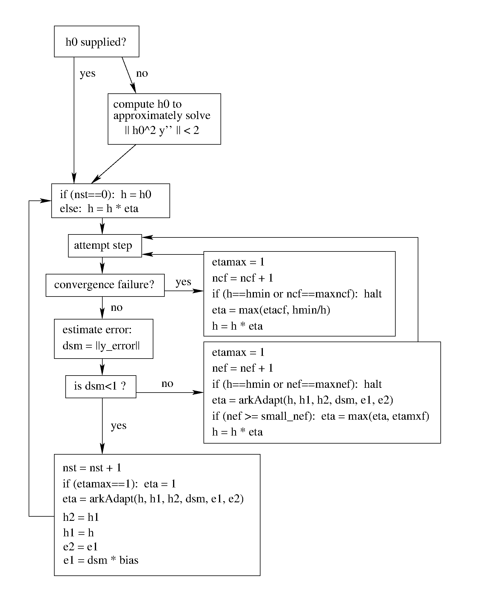
A flowchart detailing how the time steps are modified at each iteration to ensure solver convergence and successful steps is given in the figure below. Here, all norms correspond to the WRMS norm, and the error adaptivity function arkAdapt is supplied by one of the error control algorithms discussed in the subsections below.
For some problems it may be preferable to avoid small step size adjustments. This can be especially true for problems that construct a Newton Jacobian matrix or a preconditioner for a nonlinear or an iterative linear solve, where this construction is computationally expensive, and where convergence can be seriously hindered through use of an inaccurate matrix. To accommodate these scenarios, the step is left unchanged when \(\eta \in [\eta_L, \eta_U]\). The default values for this interval are \(\eta_L = 1\) and \(\eta_U = 1.0\) (so small step size adjustments are possible), and may be modified by the user.
We note that any choices for \(\eta\) (or equivalently, \(h'\)) are subsequently constrained by the optional user-supplied bounds \(h_\text{min}\) and \(h_\text{max}\). Additionally, the time-stepping algorithms in ARKODE may similarly limit \(h'\) to adhere to a user-provided “TSTOP” stopping point, \(t_\text{stop}\).
The time-stepping modules in ARKODE adapt the step size in order to attain local errors within desired tolerances of the true solution. These adaptivity algorithms estimate the prospective step size \(h'\) based on the asymptotic local error estimates (2.31). We define the values \(\varepsilon_n\), \(\varepsilon_{n-1}\) and \(\varepsilon_{n-2}\) as
corresponding to the local error estimates for three consecutive steps, \(t_{n-3} \to t_{n-2} \to t_{n-1} \to t_n\). These local error history values are all initialized to 1 upon program initialization, to accommodate the few initial time steps of a calculation where some of these error estimates have not yet been computed. With these estimates, ARKODE supports one of two approaches for temporal error control.
First, any valid implementation of the SUNAdaptController class §13.1 may be used by ARKODE’s adaptive time-stepping modules to provide a candidate error-based prospective step size \(h'\).
Second, ARKODE’s adaptive time-stepping modules currently still allow the user to define their own time step adaptivity function,
allowing for problem-specific choices, or for continued experimentation with temporal error controllers. We note that this support has been deprecated in favor of the SUNAdaptController class, and will be removed in a future release.
2.2.11.1. Multirate time step adaptivity (MRIStep)
Since multirate applications evolve on multiple time scales, MRIStep supports additional forms of temporal adaptivity. Specifically, we consider time steps at two adjacent levels, \(h^S_n > h^F_n\), where \(h^S_n\) is the step size used by MRIStep, and \(h^F_n\) is the step size used to solve the corresponding fast-time-scale IVPs in MRIStep, (2.16) and (2.18).
2.2.11.1.1. Multirate temporal controls
We consider two categories of temporal controllers that may be used within MRI methods. The first (and simplest), are “decoupled” controllers, that consist of two separate single-rate temporal controllers: one that adapts the slow time scale step size, \(h^S_n\), and the other that adapts the fast time scale step size, \(h^F_n\). As these ignore any coupling between the two time scales, these methods should work well for multirate problems where the time scales are somewhat decoupled, and that errors introduced at one scale do not “pollute” the other.
The second category of controllers that we provide are \(h^S\)-\(Tol\) multirate controllers. The basic idea is that an adaptive time integration method will attempt to adapt step sizes to control the local error within each step to achieve a requested tolerance. However, MRI methods must ask an adaptive “inner” solver to produce the stage solutions \(v_i(t_{F,i})\) and \(\tilde{v}(\tilde{t}_{F})\), that result from sub-stepping over intervals \([t_{0,i},t_{F,i}]\) or \([\tilde{t}_{0},\tilde{t}_{F}]\), respectively. Local errors within the inner integrator may accumulate, resulting in an overall inner solver error \(\varepsilon^F_n\) that exceeds the requested tolerance. If that inner solver can produce both \(v_i(t_{F,i})\) and an estimation of the accumulated error, \(\varepsilon^F_{n,approx}\), then the tolerances provided to that inner solver can be adjusted accordingly to ensure stage solutions that are within the overall tolerances requested of the outer MRI method.
To this end, we assume that the inner solver will provide accumulated errors over each fast interval having the form
where \(c(t)\) is independent of the tolerance or step size, but may vary in time. Single-scale adaptive controllers assume that the local error at a step \(n\) with step size \(h_n\) has order \(p\), i.e.,
to predict candidate values \(h_{n+1}\). We may therefore repurpose an existing single-scale controller to predict candidate values \(\text{RTOL}^F_{n+1}\) by supplying an “order” \(p=0\) and a “control parameter” \(h_n=\left(\text{RTOL}_n^F\right)\).
Thus to construct an \(h^S\)-\(Tol\) controller, we require three separate single-rate adaptivity controllers:
scontrol-H – this is a single-rate controller that adapts \(h^S_n\) within the slow integrator to achieve user-requested solution tolerances.
scontrol-Tol – this is a single-rate controller that adapts \(\text{RTOL}^F_n\) using the strategy described above.
fcontrol – this adapts time steps \(h^F_n\) within the fast integrator to achieve the current tolerance, \(\text{RTOL}^F_n\).
We note that both the decoupled and \(h^S\)-\(Tol\) controller families may be used in multirate calculations with an arbitrary number of time scales, since these focus on only one scale at a time, or on how a given time scale relates to the next-faster scale.
2.2.11.1.2. Fast temporal error estimation
MRI temporal adaptivity requires estimation of the temporal errors that arise at both the slow and fast time scales, which we denote here as \(\varepsilon^S\) and \(\varepsilon^F\), respectively. While the slow error may be estimated as \(\varepsilon^S = \|y_n - \tilde{y}_n\|\), non-intrusive approaches for estimating \(\varepsilon^F\) are more challenging. ARKODE provides several strategies to help provide this estimate, all of which assume the fast integrator is temporally adaptive and, at each of its \(m\) steps to reach \(t_n\), computes an estimate of the local temporal error, \(\varepsilon^F_{n,m}\). In this case, we assume that the fast integrator was run with the same absolute tolerances as the slow integrator, but that it may have used a potentially different relative solution tolerance, \(\text{RTOL}^F\). The fast integrator then accumulates these local error estimates using either a “maximum accumulation” strategy,
an “additive accumulation” strategy,
or using an “averaged accumulation” strategy,
where \(h_{n,m}\) is the step size that gave rise to \(\varepsilon^F_{n,m}\), \(\Delta t_{\mathcal{S}}\) denotes the elapsed time over which \(\mathcal{S}\) is taken, and the norms are taken using the tolerance-informed error-weight vector. In each case, the sum or the maximum is taken over the set of all steps \(\mathcal{S}\) since the fast error accumulator has been reset.
2.2.12. Initial step size estimation
Before time step adaptivity can be accomplished, an initial step must be taken. These values may always be provided by the user; however, if these are not provided then ARKODE will estimate a suitable choice. Typically with adaptive methods, the first step should be chosen conservatively to ensure that it succeeds both in its internal solver algorithms, and its eventual temporal error test. However, if this initial step is too conservative then its computational cost will essentially be wasted. We thus strive to construct a conservative step that will succeed while also progressing toward the eventual solution.
Before commenting on the specifics of ARKODE, we first summarize two common approaches to initial step size selection. To this end, consider a simple single-time-scale ODE,
For this, we may consider two Taylor series expansions of \(y(t_0+h)\) around the initial time,
and
where \(t_0+\tau\) is between \(t_0\) and \(t_0+h\), and \(y_0+\eta\) is on the line segment connecting \(y_0\) and \(y(t_0+h)\).
Initial step size estimation based on the first-order Taylor expansion (2.38) typically attempts to determine a step size such that an explicit Euler method for (2.37) would be sufficiently accurate, i.e.,
where we have assumed that \(y(t)\) is sufficiently differentiable, and that the norms include user-specified tolerances such that an error with norm less than one is deemed “acceptable.” Satisfying this inequality with a value of \(\frac12\) and solving for \(h_0\), we have
Finally, by estimating the time derivative with finite-differences,
we obtain
Initial step size estimation based on the simpler Taylor expansion (2.39) instead assumes that the first calculated time step should be “close” to the initial state,
where we again satisfy the inequality with a value of \(\frac12\) to obtain
Comparing the two estimates (2.40) and (2.41), we see that the former has double the number of \(f\) evaluations, but that it has a less conservative estimate of \(h_0\), particularly since we expect any valid time integration method to have at least \(\mathcal{O}(h)\) accuracy.
Of these two approaches, for calculations at a single time scale (e.g., using ARKStep), formula (2.40) is used, due to its more aggressive estimate for \(h_0\).
2.2.12.1. Initial multirate step sizes
In MRI methods, initial time step selection is complicated by the fact that not only must an initial slow step size, \(h_0^S\), be chosen, but a smaller initial step, \(h_0^F\), must also be selected. Additionally, it is typically assumed that within MRI methods, evaluation of \(f^S\) is significantly more costly than evaluation of \(f^F\), and thus we wish to construct these initial steps accordingly.
Under an assumption that conservative steps will be selected for both time scales, the error arising from temporal coupling between the slow and fast methods may be negligible. Thus, we estimate initial values of \(h^S_0\) and \(h^F_0\) independently. Due to our assumed higher cost of \(f^S\), then for the slow time scale we employ the initial estimate (2.41) for \(h^S_0\) using \(f = f^S\). Since the function \(f^F\) is assumed to be cheaper, we instead apply the estimate (2.40) for \(h^F_0\) using \(f=f^F\), and enforce an upper bound \(|h^F_0| \le \frac{|h^S_0|}{10}\).
Note
If the fast integrator does not supply its “full RHS function” \(f^F\) for the MRI method to call, then we simply initialize \(h^F_0 = \frac{h^S_0}{100}\).
2.2.13. Explicit stability
For problems that involve a nonzero explicit component, i.e. \(f^E(t,y) \ne 0\) in ARKStep or for any problem in ERKStep, explicit and ImEx Runge–Kutta methods may benefit from additional user-supplied information regarding the explicit stability region. All ARKODE adaptivity methods utilize estimates of the local error, and it is often the case that such local error control will be sufficient for method stability, since unstable steps will typically exceed the error control tolerances. However, for problems in which \(f^E(t,y)\) includes even moderately stiff components, and especially for higher-order integration methods, it may occur that a significant number of attempted steps will exceed the error tolerances. While these steps will automatically be recomputed, such trial-and-error can result in an unreasonable number of failed steps, increasing the cost of the computation. In these scenarios, a stability-based time step controller may also be useful.
Since the maximum stable explicit step for any method depends on the problem under consideration, in that the value \((h_n\lambda)\) must reside within a bounded stability region, where \(\lambda\) are the eigenvalues of the linearized operator \(\partial f^E / \partial y\), information on the maximum stable step size is not readily available to ARKODE’s time-stepping modules. However, for many problems such information may be easily obtained through analysis of the problem itself, e.g. in an advection-diffusion calculation \(f^I\) may contain the stiff diffusive components and \(f^E\) may contain the comparably nonstiff advection terms. In this scenario, an explicitly stable step \(h_\text{exp}\) would be predicted as one satisfying the Courant-Friedrichs-Lewy (CFL) stability condition for the advective portion of the problem,
where \(\Delta x\) is the spatial mesh size and \(\lambda\) is the fastest advective wave speed.
In these scenarios, a user may supply a routine to predict this maximum explicitly stable step size, \(|h_\text{exp}|\). If a value for \(|h_\text{exp}|\) is supplied, it is compared against the value resulting from the local error controller, \(|h_\text{acc}|\), and the eventual time step used will be limited accordingly,
Here the explicit stability step factor \(c>0\) (often called the “CFL number”) defaults to \(1/2\) but may be modified by the user.
2.2.14. Fixed time stepping
While most of the time-stepping modules are designed for tolerance-based time step adaptivity, they additionally support a “fixed-step” mode. This mode is typically used for debugging purposes, for verification against hand-coded methods, or for problems where the time steps should be chosen based on other problem-specific information. In this mode, all internal time step adaptivity is disabled:
temporal error control is disabled,
nonlinear or linear solver non-convergence will result in an error (instead of a step size adjustment),
no check against an explicit stability condition is performed.
Note
Since temporal error based adaptive time-stepping is known to ruin the conservation property of SPRK methods, SPRKStep employs a fixed time-step size by default.
Note
Any methods that do not provide an embedding are required to be run in fixed-step mode.
Additional information on this mode is provided in the section ARKODE Optional Inputs.
2.2.15. Algebraic solvers
When solving a problem involving either an implicit component (e.g., in ARKStep with \(f^I(t,y) \ne 0\), or in MRIStep with a solve-decoupled implicit slow stage), or a non-identity mass matrix (\(M(t) \ne I\) in ARKStep), systems of linear or nonlinear algebraic equations must be solved at each stage and/or step of the method. This section therefore focuses on the variety of mathematical methods provided in the ARKODE infrastructure for such problems, including nonlinear solvers, linear solvers, preconditioners, iterative solver error control, implicit predictors, and techniques used for simplifying the above solves when using different classes of mass-matrices.
2.2.15.1. Nonlinear solver methods
Methods with an implicit partition require solving implicit systems of the form
In order to maximize solver efficiency, we define this root-finding problem differently based on the type of mass-matrix supplied by the user.
In the case that \(M=I\) within ARKStep, we define the residual as
(2.43)\[G(z_i) \equiv z_i - h_n A^I_{i,i} f^I(t^I_{n,i}, z_i) - a_i,\]where we have the data
\[a_i \equiv y_{n-1} + h_n \sum_{j=1}^{i-1} \left[ A^E_{i,j} f^E(t^E_{n,j}, z_j) + A^I_{i,j} f^I(t^I_{n,j}, z_j) \right].\]In the case of non-identity mass matrix \(M\ne I\) within ARKStep, but where \(M\) is independent of \(t\), we define the residual as
(2.44)\[G(z_i) \equiv M z_i - h_n A^I_{i,i} f^I(t^I_{n,i}, z_i) - a_i,\]where we have the data
\[a_i \equiv M y_{n-1} + h_n \sum_{j=1}^{i-1} \left[ A^E_{i,j} f^E(t^E_{n,j}, z_j) + A^I_{i,j} f^I(t^I_{n,j}, z_j) \right].\]Note
This form of residual, as opposed to \(G(z_i) = z_i - h_n A^I_{i,i} \hat{f}^I(t^I_{n,i}, z_i) - a_i\) (with \(a_i\) defined appropriately), removes the need to perform the nonlinear solve with right-hand side function \(\hat{f}^I=M^{-1}\,f^I\), as that would require a linear solve with \(M\) at every evaluation of the implicit right-hand side routine.
In the case of ARKStep with \(M\) dependent on \(t\), we define the residual as
(2.45)\[G(z_i) \equiv M(t^I_{n,i}) (z_i - a_i) - h_n A^I_{i,i} f^I(t^I_{n,i}, z_i)\]where we have the data
\[a_i \equiv y_{n-1} + h_n \sum_{j=1}^{i-1} \left[ A^E_{i,j} \hat{f}^E(t^E_{n,j}, z_j) + A^I_{i,j} \hat{f}^I(t^I_{n,j}, z_j) \right].\]Note
As above, this form of the residual is chosen to remove excessive mass-matrix solves from the nonlinear solve process.
Similarly, in MRIStep (that always assumes \(M=I\)), MRI-GARK and IMEX-MRI-GARK methods have the residual
(2.46)\[G(z_i) \equiv z_i - h^S_n \left(\sum_{k\geq 1} \frac{\Gamma_{i,i,k}}{k}\right) f^I(t_{n,i}^S, z_i) - a_i = 0\]where
\[a_i \equiv z_{i-1} + h^S_n \sum_{j=1}^{i-1} \left(\sum_{k\geq 1} \frac{\Gamma_{i,j,k}}{k}\right)f^I(t_{n,j}^S, z_j).\]IMEX-MRI-SR methods have the residual
(2.47)\[G(z_i) \equiv z_i - h^S_n \Gamma_{i,i} f^I(t_{n,i}^S, z_i) - a_i = 0\]where
\[a_i \equiv z_{i-1} + h^S_n \sum_{j=1}^{i-1} \Gamma_{i,j} f^I(t_{n,j}^S, z_j).\]
Upon solving for \(z_i\), method stages must store \(f^E(t^E_{n,j}, z_i)\) and \(f^I(t^I_{n,j}, z_i)\). It is possible to compute the latter without evaluating \(f^I\) after each nonlinear solve. Consider, for example, (2.43) which implies
(2.48)\[f^I(t^I_{n,j}, z_i) = \frac{z_i - a_i}{h_n A^I_{i,i}}\]
when \(z_i\) is the exact root, and similar relations hold for non-identity
mass matrices. This optimization can be enabled by ARKodeSetDeduceImplicitRhs()
with the second argument in either function set to SUNTRUE. Another factor to
consider when using this option is the amplification of errors from the
nonlinear solver to the stages. In (2.48), nonlinear
solver errors in \(z_i\) are scaled by \(1 / (h_n A^I_{i,i})\). By
evaluating \(f^I\) on \(z_i\), errors are scaled roughly by the Lipshitz
constant \(L\) of the problem. If \(h_n A^I_{i,i} L > 1\), which is
often the case when using implicit methods, it may be more accurate to use
(2.48). Additional details are discussed in
[131].
In each of the above nonlinear residual functions, if \(f^I(t,y)\) depends nonlinearly on \(y\) then (2.42) corresponds to a nonlinear system of equations; if instead \(f^I(t,y)\) depends linearly on \(y\) then this is a linear system of equations.
To solve each of the above root-finding problems ARKODE leverages SUNNonlinearSolver modules from the underlying SUNDIALS infrastructure (see section §11). By default, ARKODE selects a variant of Newton’s method,
where \(m\) is the Newton iteration index, and the Newton update \(\delta^{(m+1)}\) in turn requires the solution of the Newton linear system
in which
within ARKStep, or
within MRIStep.
In addition to Newton-based nonlinear solvers, the SUNDIALS SUNNonlinearSolver interface allows solvers of fixed-point type. These generally implement a fixed point iteration for solving an implicit stage \(z_i\),
Unlike with Newton-based nonlinear solvers, fixed-point iterations generally do not require the solution of a linear system involving the Jacobian of \(f\) at each iteration.
Finally, if the user specifies that \(f^I(t,y)\) depends linearly on \(y\) in ARKStep or MRIStep and if the Newton-based SUNNonlinearSolver module is used, then the problem (2.42) will be solved using only a single Newton iteration. In this case, an additional user-supplied argument indicates whether this Jacobian is time-dependent or not, signaling whether the Jacobian or preconditioner needs to be recomputed at each stage or time step, or if it can be reused throughout the full simulation.
The optimal choice of solver (Newton vs fixed-point) is highly problem dependent. Since fixed-point solvers do not require the solution of linear systems involving the Jacobian of \(f\), each iteration may be significantly less costly than their Newton counterparts. However, this can come at the cost of slower convergence (or even divergence) in comparison with Newton-like methods. While a Newton-based iteration is the default solver in ARKODE due to its increased robustness on very stiff problems, we strongly recommend that users also consider the fixed-point solver when attempting a new problem.
For either the Newton or fixed-point solvers, it is well-known that both the efficiency and robustness of the algorithm intimately depend on the choice of a good initial guess. The initial guess for these solvers is a prediction \(z_i^{(0)}\) that is computed explicitly from previously-computed data (e.g. \(y_{n-2}\), \(y_{n-1}\), and \(z_j\) where \(j<i\)). Additional information on the specific predictor algorithms is provided in section §2.2.15.5.
2.2.15.2. Linear solver methods
When a Newton-based method is chosen for solving each nonlinear system, a linear system of equations must be solved at each nonlinear iteration. For this solve ARKODE leverages another component of the shared SUNDIALS infrastructure, the “SUNLinearSolver,” described in section §10. These linear solver modules are grouped into two categories: matrix-based linear solvers and matrix-free iterative linear solvers. ARKODE’s interfaces for linear solves of these types are described in the subsections below.
2.2.15.2.1. Matrix-based linear solvers
In the case that a matrix-based linear solver is selected, a modified Newton iteration is utilized. In a modified Newton iteration, the matrix \({\mathcal A}\) is held fixed for multiple Newton iterations. More precisely, each Newton iteration is computed from the modified equation
in which
or
Here, the solution \(\tilde{z}\), time \(\tilde{t}\), and step size \(\tilde{h}\) upon which the modified equation rely, are merely values of these quantities from a previous iteration. In other words, the matrix \(\tilde{\mathcal A}\) is only computed rarely, and reused for repeated solves. As described below in section §2.2.15.2.3, the frequency at which \(\tilde{\mathcal A}\) is recomputed defaults to 20 time steps, but may be modified by the user.
When using the dense and band SUNMatrix objects for the linear systems (2.54), the Jacobian \(J\) may be supplied by a user routine, or approximated internally with finite-differences. In the case of differencing, we use the standard approximation
where \(e_j\) is the \(j\)-th unit vector, and the increments \(\sigma_j\) are given by
Here \(U\) is the unit roundoff, \(\sigma_0\) is a small dimensionless value, and \(w_j\) is the error weight defined in (2.29). In the dense case, this approach requires \(N\) evaluations of \(f^I\), one for each column of \(J\). In the band case, the columns of \(J\) are computed in groups, using the Curtis-Powell-Reid algorithm, with the number of \(f^I\) evaluations equal to the matrix bandwidth.
We note that with sparse and user-supplied SUNMatrix objects, the Jacobian must be supplied by a user routine.
2.2.15.2.2. Matrix-free iterative linear solvers
In the case that a matrix-free iterative linear solver is chosen, an inexact Newton iteration is utilized. Here, the matrix \({\mathcal A}\) is not itself constructed since the algorithms only require the product of this matrix with a given vector. Additionally, each Newton system (2.50) is not solved completely, since these linear solvers are iterative (hence the “inexact” in the name). As a result. for these linear solvers \({\mathcal A}\) is applied in a matrix-free manner,
The mass matrix-vector products \(Mv\) must be provided through a user-supplied routine; the Jacobian matrix-vector products \(Jv\) are obtained by either calling an optional user-supplied routine, or through a finite difference approximation to the directional derivative:
where we use the increment \(\sigma = 1/\|v\|\) to ensure that \(\|\sigma v\| = 1\).
As with the modified Newton method that reused \({\mathcal A}\) between solves, the inexact Newton iteration may also recompute the preconditioner \(P\) infrequently to balance the high costs of matrix construction and factorization against the reduced convergence rate that may result from a stale preconditioner.
2.2.15.2.3. Updating the linear solver
In cases where recomputation of the Newton matrix \(\tilde{\mathcal A}\) or preconditioner \(P\) is lagged, these structures will be recomputed only in the following circumstances:
when starting the problem,
when more than \(msbp = 20\) steps have been taken since the last update (this value may be modified by the user),
when the value \(\tilde{\gamma}\) of \(\gamma\) at the last update satisfies \(\left|\gamma/\tilde{\gamma} - 1\right| > \Delta\gamma_{max} = 0.2\) (this value may be modified by the user),
when a non-fatal convergence failure just occurred,
when an error test failure just occurred, or
if the problem is linearly implicit and \(\gamma\) has changed by a factor larger than 100 times machine epsilon.
When an update of \(\tilde{\mathcal A}\) or \(P\) occurs, it may or may not involve a reevaluation of \(J\) (in \(\tilde{\mathcal A}\)) or of Jacobian data (in \(P\)), depending on whether errors in the Jacobian were the likely cause for the update. Reevaluating \(J\) (or instructing the user to update \(P\)) occurs when:
starting the problem,
more than \(msbj=50\) steps have been taken since the last evaluation (this value may be modified by the user),
a convergence failure occurred with an outdated matrix, and the value \(\tilde{\gamma}\) of \(\gamma\) at the last update satisfies \(\left|\gamma/\tilde{\gamma} - 1\right| > 0.2\),
a convergence failure occurred that forced a step size reduction, or
if the problem is linearly implicit and \(\gamma\) has changed by a factor larger than 100 times machine epsilon.
However, for linear solvers and preconditioners that do not rely on costly matrix construction and factorization operations (e.g. when using a geometric multigrid method as preconditioner), it may be more efficient to update these structures more frequently than the above heuristics specify, since the increased rate of linear/nonlinear solver convergence may more than account for the additional cost of Jacobian/preconditioner construction. To this end, a user may specify that the system matrix \({\mathcal A}\) and/or preconditioner \(P\) should be recomputed more frequently.
As will be further discussed in section §2.2.15.4, in the case of most Krylov methods, preconditioning may be applied on the left, right, or on both sides of \({\mathcal A}\), with user-supplied routines for the preconditioner setup and solve operations.
2.2.15.3. Iteration Error Control
2.2.15.3.1. Nonlinear iteration error control
ARKODE provides a customized stopping test to the SUNNonlinearSolver module used for solving equation (2.42). This test is related to the temporal local error test, with the goal of keeping the nonlinear iteration errors from interfering with local error control. Denoting the final computed value of each stage solution as \(z_i^{(m)}\), and the true stage solution solving (2.42) as \(z_i\), we want to ensure that the iteration error \(z_i - z_i^{(m)}\) is “small” (recall that a norm less than 1 is already considered within an acceptable tolerance).
To this end, we first estimate the linear convergence rate \(R_i\) of the nonlinear iteration. We initialize \(R_i=1\), and reset it to this value whenever \(\tilde{\mathcal A}\) or \(P\) are updated. After computing a nonlinear correction \(\delta^{(m)} = z_i^{(m)} - z_i^{(m-1)}\), if \(m>0\) we update \(R_i\) as
where the default factor \(c_r=0.3\) is user-modifiable.
Let \(y_n^{(m)}\) denote the time-evolved solution constructed using our approximate nonlinear stage solutions, \(z_i^{(m)}\), and let \(y_n^{(\infty)}\) denote the time-evolved solution constructed using exact nonlinear stage solutions. We then use the estimate
Therefore our convergence (stopping) test for the nonlinear iteration for each stage is
where the factor \(\epsilon\) has default value 0.1. We default to a maximum of 3 nonlinear iterations. We also declare the nonlinear iteration to be divergent if any of the ratios
with \(m>0\), where \(r_{div}\) defaults to 2.3. If convergence fails in the nonlinear solver with \({\mathcal A}\) current (i.e., not lagged), we reduce the step size \(h_n\) by a factor of \(\eta_{cf}=0.25\). The integration will be halted after \(max_{ncf}=10\) convergence failures, or if a convergence failure occurs with \(h_n = h_\text{min}\). However, since the nonlinearity of (2.42) may vary significantly based on the problem under consideration, these default constants may all be modified by the user.
2.2.15.3.2. Linear iteration error control
When a Krylov method is used to solve the linear Newton systems (2.50), its errors must also be controlled. To this end, we approximate the linear iteration error in the solution vector \(\delta^{(m)}\) using the preconditioned residual vector, e.g. \(r = P{\mathcal A}\delta^{(m)} + PG\) for the case of left preconditioning (the role of the preconditioner is further elaborated in the next section). In an attempt to ensure that the linear iteration errors do not interfere with the nonlinear solution error and local time integration error controls, we require that the norm of the preconditioned linear residual satisfies
Here \(\epsilon\) is the same value as that is used above for the nonlinear error control. The factor of 10 is used to ensure that the linear solver error does not adversely affect the nonlinear solver convergence. Smaller values for the parameter \(\epsilon_L\) are typically useful for strongly nonlinear or very stiff ODE systems, while easier ODE systems may benefit from a value closer to 1. The default value is \(\epsilon_L = 0.05\), which may be modified by the user. We note that for linearly implicit problems the tolerance (2.60) is similarly used for the single Newton iteration.
2.2.15.4. Preconditioning
When using an inexact Newton method to solve the nonlinear system (2.42), an iterative method is used repeatedly to solve linear systems of the form \({\mathcal A}x = b\), where \(x\) is a correction vector and \(b\) is a residual vector. If this iterative method is one of the scaled preconditioned iterative linear solvers supplied with SUNDIALS, their efficiency may benefit tremendously from preconditioning. A system \({\mathcal A}x=b\) can be preconditioned using any one of:
These Krylov iterative methods are then applied to a system with the matrix \(P^{-1}{\mathcal A}\), \({\mathcal A}P^{-1}\), or \(P_L^{-1} {\mathcal A} P_R^{-1}\), instead of \({\mathcal A}\). In order to improve the convergence of the Krylov iteration, the preconditioner matrix \(P\), or the product \(P_L P_R\) in the third case, should in some sense approximate the system matrix \({\mathcal A}\). Simultaneously, in order to be cost-effective the matrix \(P\) (or matrices \(P_L\) and \(P_R\)) should be reasonably efficient to evaluate and solve. Finding an optimal point in this trade-off between rapid convergence and low cost can be quite challenging. Good choices are often problem-dependent (for example, see [25] for an extensive study of preconditioners for reaction-transport systems).
Most of the iterative linear solvers supplied with SUNDIALS allow for all three types of preconditioning (left, right or both), although for non-symmetric matrices \({\mathcal A}\) we know of few situations where preconditioning on both sides is superior to preconditioning on one side only (with the product \(P = P_L P_R\)). Moreover, for a given preconditioner matrix, the merits of left vs. right preconditioning are unclear in general, so we recommend that the user experiment with both choices. Performance can differ between these since the inverse of the left preconditioner is included in the linear system residual whose norm is being tested in the Krylov algorithm. As a rule, however, if the preconditioner is the product of two matrices, we recommend that preconditioning be done either on the left only or the right only, rather than using one factor on each side. An exception to this rule is the PCG solver, that itself assumes a symmetric matrix \({\mathcal A}\), since the PCG algorithm in fact applies the single preconditioner matrix \(P\) in both left/right fashion as \(P^{-1/2} {\mathcal A} P^{-1/2}\).
Typical preconditioners are based on approximations to the system Jacobian, \(J = \partial f^I / \partial y\). Since the Newton iteration matrix involved is \({\mathcal A} = M - \gamma J\), any approximation \(\bar{J}\) to \(J\) yields a matrix that is of potential use as a preconditioner, namely \(P = M - \gamma \bar{J}\). Because the Krylov iteration occurs within a Newton iteration and further also within a time integration, and since each of these iterations has its own test for convergence, the preconditioner may use a very crude approximation, as long as it captures the dominant numerical features of the system. We have found that the combination of a preconditioner with the Newton-Krylov iteration, using even a relatively poor approximation to the Jacobian, can be surprisingly superior to using the same matrix without Krylov acceleration (i.e., a modified Newton iteration), as well as to using the Newton-Krylov method with no preconditioning.
2.2.15.5. Implicit predictors
For problems with implicit components, a prediction algorithm is employed for constructing the initial guesses for each implicit Runge–Kutta stage, \(z_i^{(0)}\). As is well-known with nonlinear solvers, the selection of a good initial guess can have dramatic effects on both the speed and robustness of the solve, making the difference between rapid quadratic convergence versus divergence of the iteration. To this end, a variety of prediction algorithms are provided. In each case, the stage guesses \(z_i^{(0)}\) are constructed explicitly using readily-available information, including the previous step solutions \(y_{n-1}\) and \(y_{n-2}\), as well as any previous stage solutions \(z_j, \quad j<i\). In most cases, prediction is performed by constructing an interpolating polynomial through existing data, which is then evaluated at the desired stage time to provide an inexpensive but (hopefully) reasonable prediction of the stage solution. Specifically, for most Runge–Kutta methods each stage solution satisfies
(similarly for MRI methods \(z_i \approx y(t^S_{n,i})\)), so by constructing an interpolating polynomial \(p_q(t)\) through a set of existing data, the initial guess at stage solutions may be approximated as
As the stage times for MRI stages and implicit ARK and DIRK stages usually have non-negative abscissae (i.e., \(c_j^I > 0\)), it is typically the case that \(t^I_{n,j}\) (resp., \(t^S_{n,j}\)) is outside of the time interval containing the data used to construct \(p_q(t)\), hence (2.61) will correspond to an extrapolant instead of an interpolant. The dangers of using a polynomial interpolant to extrapolate values outside the interpolation interval are well-known, with higher-order polynomials and predictions further outside the interval resulting in the greatest potential inaccuracies.
The prediction algorithms available in ARKODE therefore construct a variety of interpolants \(p_q(t)\), having different polynomial order and using different interpolation data, to support “optimal” choices for different types of problems, as described below. We note that due to the structural similarities between implicit ARK and DIRK stages in ARKStep, and solve-decoupled implicit stages in MRIStep, we use the ARKStep notation throughout the remainder of this section, but each statement equally applies to MRIStep (unless otherwise noted).
2.2.15.5.1. Trivial predictor
The so-called “trivial predictor” is given by the formula
While this piecewise-constant interpolant is clearly not a highly accurate candidate for problems with time-varying solutions, it is often the most robust approach for highly stiff problems, or for problems with implicit constraints whose violation may cause illegal solution values (e.g. a negative density or temperature).
2.2.15.5.2. Maximum order predictor
At the opposite end of the spectrum, ARKODE’s interpolation modules discussed in section §2.2.2 can be used to construct a higher-order polynomial interpolant, \(p_q(t)\). The implicit stage predictor is computed through evaluating the highest-degree-available interpolant at each stage time \(t^I_{n,i}\).
2.2.15.5.3. Variable order predictor
This predictor attempts to use higher-degree polynomials \(p_q(t)\) for predicting earlier stages, and lower-degree interpolants for later stages. It uses the same interpolation module as described above, but chooses the polynomial degree adaptively based on the stage index \(i\), under the assumption that the stage times are increasing, i.e. \(c^I_j < c^I_k\) for \(j<k\):
2.2.15.5.4. Cutoff order predictor
This predictor follows a similar idea as the previous algorithm, but monitors the actual stage times to determine the polynomial interpolant to use for prediction. Denoting \(\tau = c_i^I \dfrac{h_n}{h_{n-1}}\), the polynomial degree \(q_i\) is chosen as:
2.2.15.5.5. Bootstrap predictor (\(M=I\) only) – deprecated
This predictor does not use any information from the preceding step, instead using information only within the current step \([t_{n-1},t_n]\). In addition to using the solution and ODE right-hand side function, \(y_{n-1}\) and \(f(t_{n-1},y_{n-1})\), this approach uses the right-hand side from a previously computed stage solution in the same step, \(f(t_{n-1}+c^I_j h,z_j)\) to construct a quadratic Hermite interpolant for the prediction. If we define the constants \(\tilde{h} = c^I_j h\) and \(\tau = c^I_i h\), the predictor is given by
For stages without a nonzero preceding stage time, i.e. \(c^I_j\ne 0\) for \(j<i\), this method reduces to using the trivial predictor \(z_i^{(0)} = y_{n-1}\). For stages having multiple preceding nonzero \(c^I_j\), we choose the stage having largest \(c^I_j\) value, to minimize the level of extrapolation used in the prediction.
We note that in general, each stage solution \(z_j\) has significantly worse accuracy than the time step solutions \(y_{n-1}\), due to the difference between the stage order and the method order in Runge–Kutta methods. As a result, the accuracy of this predictor will generally be rather limited, but it is provided for problems in which this increased stage error is better than the effects of extrapolation far outside of the previous time step interval \([t_{n-2},t_{n-1}]\).
Although this approach could be used with non-identity mass matrix, support for that mode is not currently implemented, so selection of this predictor in the case of a non-identity mass matrix will result in use of the trivial predictor.
Note
This predictor has been deprecated, and will be removed from a future release.
2.2.15.5.6. Minimum correction predictor (ARKStep, \(M=I\) only) – deprecated
The final predictor is not interpolation based; instead it utilizes all existing stage information from the current step to create a predictor containing all but the current stage solution. Specifically, as discussed in equations (2.8) and (2.42), each stage solves a nonlinear equation
This prediction method merely computes the predictor \(z_i\) as
Again, although this approach could be used with non-identity mass matrix, support for that mode is not currently implemented, so selection of this predictor in the case of a non-identity mass matrix will result in use of the trivial predictor.
Note
This predictor has been deprecated, and will be removed from a future release.
2.2.15.6. Mass matrix solver (ARKStep only)
Within the ARKStep algorithms described above, there are multiple locations where a matrix-vector product
or a linear solve
is required.
Of course, for problems in which \(M=I\) both of these operators are trivial. However for problems with non-identity mass matrix, these linear solves (2.63) may be handled using any valid SUNLinearSolver module, in the same manner as described in the section §2.2.15.2 for solving the linear Newton systems.
For ERK methods involving non-identity mass matrix, even though calculation of individual stages does not require an algebraic solve, both of the above operations (matrix-vector product, and mass matrix solve) may be required within each time step. Therefore, for these users we recommend reading the rest of this section as it pertains to ARK methods, with the obvious simplification that since \(f^E=f\) and \(f^I=0\) no Newton or fixed-point nonlinear solve, and no overall system linear solve, is involved in the solution process.
At present, for DIRK and ARK problems using a matrix-based solver for
the Newton nonlinear iterations, the type of matrix (dense, band,
sparse, or custom) for the Jacobian matrix \(J\) must match the
type of mass matrix \(M\), since these are combined to form the
Newton system matrix \(\tilde{\mathcal A}\). When matrix-based
methods are employed, the user must supply a routine to compute
\(M(t)\) in the appropriate form to match the structure of
\({\mathcal A}\), with a user-supplied routine of type
ARKLsMassFn(). This matrix structure is used internally to
perform any requisite mass matrix-vector products (2.62).
When matrix-free methods are selected, a routine must be supplied to perform the mass-matrix-vector product, \(Mv\). As with iterative solvers for the Newton systems, preconditioning may be applied to aid in solution of the mass matrix systems (2.63). When using an iterative mass matrix linear solver, we require that the norm of the preconditioned linear residual satisfies
where again, \(\epsilon\) is the nonlinear solver tolerance parameter from (2.58). When using iterative system and mass matrix linear solvers, \(\epsilon_L\) may be specified separately for both tolerances (2.60) and (2.64).
In the algorithmic descriptions above there are five locations where a linear solve of the form (2.63) is required: (a) at each iteration of a fixed-point nonlinear solve, (b) in computing the Runge–Kutta right-hand side vectors \(\hat{f}^E_i\) and \(\hat{f}^I_i\), (c) in constructing the time-evolved solution \(y_n\), (d) in estimating the local temporal truncation error, and (e) in constructing predictors for the implicit solver iteration (see section §2.2.15.5.2). We note that different nonlinear solver approaches (i.e., Newton vs fixed-point) and different types of mass matrices (i.e., time-dependent versus fixed) result in different subsets of the above operations. We discuss each of these in the bullets below.
When using a fixed-point nonlinear solver, at each fixed-point iteration we must solve
\[M(t^I_{n,i})\, z_i^{(m+1)} = G\left(z_i^{(m)}\right), \quad m=0,1,\ldots\]for the new fixed-point iterate, \(z_i^{(m+1)}\).
In the case of a time-dependent mass matrix, to construct the Runge–Kutta right-hand side vectors we must solve
\[M(t^E_{n,i}) \hat{f}^{E}_i \ = \ f^{E}(t^E_{n,i},z_i) \quad\text{and}\quad M(t^I_{n,i}) \hat{f}^{I}_j \ = \ f^{I}(t^I_{n,i},z_i)\]for the vectors \(\hat{f}^{E}_i\) and \(\hat{f}^{I}_i\).
For fixed mass matrices, we construct the time-evolved solution \(y_n\) from equation (2.8) by solving
\[\begin{split}&M y_n \ = \ M y_{n-1} + h_n \sum_{i=1}^{s} \left( b^E_i f^E(t^E_{n,i}, z_i) + b^I_i f^I(t^I_{n,i}, z_i)\right), \\ \Leftrightarrow \qquad & \\ &M (y_n -y_{n-1}) \ = \ h_n \sum_{i=1}^{s} \left(b^E_i f^E(t^E_{n,i}, z_i) + b^I_i f^I(t^I_{n,i}, z_i)\right), \\ \Leftrightarrow \qquad & \\ &M \nu \ = \ h_n \sum_{i=1}^{s} \left(b^E_i f^E(t^E_{n,i}, z_i) + b^I_i f^I(t^I_{n,i}, z_i)\right),\end{split}\]for the update \(\nu = y_n - y_{n-1}\).
Similarly, we compute the local temporal error estimate \(T_n\) from equation (2.32) by solving systems of the form
(2.65)\[M\, T_n = h \sum_{i=1}^{s} \left[ \left(b^E_i - \tilde{b}^E_i\right) f^E(t^E_{n,i}, z_i) + \left(b^I_i - \tilde{b}^I_i\right) f^I(t^I_{n,i}, z_i) \right].\]For problems with either form of non-identity mass matrix, in constructing dense output and implicit predictors of degree 2 or higher (see the section §2.2.15.5.2 above), we compute the derivative information \(\hat{f}_k\) from the equation
\[M(t_n) \hat{f}_n = f^E(t_n, y_n) + f^I(t_n, y_n).\]
In total, for problems with fixed mass matrix, we require only two mass-matrix linear solves (2.63) per attempted time step, with one more upon completion of a time step that meets the solution accuracy requirements. When fixed time-stepping is used (\(h_n=h\)), the solve (2.65) is not performed at each attempted step.
Similarly, for problems with time-dependent mass matrix, we require \(2s\) mass-matrix linear solves (2.63) per attempted step, where \(s\) is the number of stages in the ARK method (only half of these are required for purely explicit or purely implicit problems, (2.9) or (2.10)), with one more upon completion of a time step that meets the solution accuracy requirements.
In addition to the above totals, when using a fixed-point nonlinear solver (assumed to require \(m\) iterations), we will need an additional \(ms\) mass-matrix linear solves (2.63) per attempted time step (but zero linear solves with the system Jacobian).
2.2.16. Rootfinding
ARKODE also supports a rootfinding feature, in that while integrating the IVP (2.5), these can also find the roots of a set of user-defined functions \(g_i(t,y)\) that depend on \(t\) and the solution vector \(y = y(t)\). The number of these root functions is arbitrary, and if more than one \(g_i\) is found to have a root in any given interval, the various root locations are found and reported in the order that they occur on the \(t\) axis, in the direction of integration.
Generally, this rootfinding feature finds only roots of odd multiplicity, corresponding to changes in sign of \(g_i(t, y(t))\), denoted \(g_i(t)\) for short. If a user root function has a root of even multiplicity (no sign change), it will almost certainly be missed due to the realities of floating-point arithmetic. If such a root is desired, the user should reformulate the root function so that it changes sign at the desired root.
The basic scheme used is to check for sign changes of any \(g_i(t)\) over each time step taken, and then (when a sign change is found) to home in on the root (or roots) with a modified secant method [77]. In addition, each time \(g\) is evaluated, ARKODE checks to see if \(g_i(t) = 0\) exactly, and if so it reports this as a root. However, if an exact zero of any \(g_i\) is found at a point \(t\), ARKODE computes \(g(t+\delta)\) for a small increment \(\delta\), slightly further in the direction of integration, and if any \(g_i(t+\delta) = 0\) also, ARKODE stops and reports an error. This way, each time ARKODE takes a time step, it is guaranteed that the values of all \(g_i\) are nonzero at some past value of \(t\), beyond which a search for roots is to be done.
At any given time in the course of the time-stepping, after suitable checking and adjusting has been done, ARKODE has an interval \((t_\text{lo}, t_\text{hi}]\) in which roots of the \(g_i(t)\) are to be sought, such that \(t_\text{hi}\) is further ahead in the direction of integration, and all \(g_i(t_\text{lo}) \ne 0\). The endpoint \(t_\text{hi}\) is either \(t_n\), the end of the time step last taken, or the next requested output time \(t_\text{out}\) if this comes sooner. The endpoint \(t_\text{lo}\) is either \(t_{n-1}\), or the last output time \(t_\text{out}\) (if this occurred within the last step), or the last root location (if a root was just located within this step), possibly adjusted slightly toward \(t_n\) if an exact zero was found. The algorithm checks \(g(t_\text{hi})\) for zeros, and it checks for sign changes in \((t_\text{lo}, t_\text{hi})\). If no sign changes are found, then either a root is reported (if some \(g_i(t_\text{hi}) = 0\)) or we proceed to the next time interval (starting at \(t_\text{hi}\)). If one or more sign changes were found, then a loop is entered to locate the root to within a rather tight tolerance, given by
Whenever sign changes are seen in two or more root functions, the one deemed most likely to have its root occur first is the one with the largest value of \(\left|g_i(t_\text{hi})\right| / \left| g_i(t_\text{hi}) - g_i(t_\text{lo})\right|\), corresponding to the closest to \(t_\text{lo}\) of the secant method values. At each pass through the loop, a new value \(t_\text{mid}\) is set, strictly within the search interval, and the values of \(g_i(t_\text{mid})\) are checked. Then either \(t_\text{lo}\) or \(t_\text{hi}\) is reset to \(t_\text{mid}\) according to which subinterval is found to have the sign change. If there is none in \((t_\text{lo}, t_\text{mid})\) but some \(g_i(t_\text{mid}) = 0\), then that root is reported. The loop continues until \(\left|t_\text{hi} - t_\text{lo} \right| < \tau\), and then the reported root location is \(t_\text{hi}\). In the loop to locate the root of \(g_i(t)\), the formula for \(t_\text{mid}\) is
where \(\alpha\) is a weight parameter. On the first two passes through the loop, \(\alpha\) is set to 1, making \(t_\text{mid}\) the secant method value. Thereafter, \(\alpha\) is reset according to the side of the subinterval (low vs high, i.e. toward \(t_\text{lo}\) vs toward \(t_\text{hi}\)) in which the sign change was found in the previous two passes. If the two sides were opposite, \(\alpha\) is set to 1. If the two sides were the same, \(\alpha\) is halved (if on the low side) or doubled (if on the high side). The value of \(t_\text{mid}\) is closer to \(t_\text{lo}\) when \(\alpha < 1\) and closer to \(t_\text{hi}\) when \(\alpha > 1\). If the above value of \(t_\text{mid}\) is within \(\tau /2\) of \(t_\text{lo}\) or \(t_\text{hi}\), it is adjusted inward, such that its fractional distance from the endpoint (relative to the interval size) is between 0.1 and 0.5 (with 0.5 being the midpoint), and the actual distance from the endpoint is at least \(\tau/2\).
Finally, we note that when running in parallel, ARKODE’s rootfinding module assumes that the entire set of root defining functions \(g_i(t,y)\) is replicated on every MPI rank. Since in these cases the vector \(y\) is distributed across ranks, it is the user’s responsibility to perform any necessary communication to ensure that \(g_i(t,y)\) is identical on each rank.
2.2.17. Inequality Constraints
The ARKStep and ERKStep modules in ARKODE permit the user to impose optional inequality constraints on individual components of the solution vector \(y\). Any of the following four constraints can be imposed: \(y_i > 0\), \(y_i < 0\), \(y_i \geq 0\), or \(y_i \leq 0\). The constraint satisfaction is tested after a successful step and before the error test. If any constraint fails, the step size is reduced and a flag is set to update the Jacobian or preconditioner if applicable. Rather than cutting the step size by some arbitrary factor, ARKODE estimates a new step size \(h'\) using a linear approximation of the components in \(y\) that failed the constraint test (including a safety factor of 0.9 to cover the strict inequality case). If a step fails to satisfy the constraints 10 times (a value which may be modified by the user) within a step attempt, or fails with the minimum step size, then the integration is halted and an error is returned. In this case the user may need to employ other strategies as discussed in §2.4.3.2 to satisfy the inequality constraints.
2.2.18. Relaxation Methods
When the solution of (2.5) is conservative or dissipative with respect to a smooth convex function \(\xi(y(t))\), it is desirable to have the numerical method preserve these properties. That is \(\xi(y_n) = \xi(y_{n-1}) = \ldots = \xi(y_{0})\) for conservative systems and \(\xi(y_n) \leq \xi(y_{n-1})\) for dissipative systems. For examples of such problems, see the references below and the citations there in.
For such problems, ARKODE supports relaxation methods [91, 97, 115, 116] applied to ERK, DIRK, or ARK methods to ensure dissipation or preservation of the global function. The relaxed solution is given by
where \(d\) is the update to \(y_n\) (i.e., \(h_n \sum_{i=1}^{s}(b^E_i \hat{f}^E_i + b^I_i \hat{f}^I_i)\) for ARKStep and \(h_n \sum_{i=1}^{s} b_i f_i\) for ERKStep) and \(r\) is the relaxation factor selected to ensure conservation or dissipation. Given an ERK, DIRK, or ARK method of at least second order with non-negative solution weights (i.e., \(b_i \geq 0\) for ERKStep or \(b^E_i \geq 0\) and \(b^I_i \geq 0\) for ARKStep), the factor \(r\) is computed by solving the auxiliary scalar nonlinear system
at the end of each time step. The estimated change in \(\xi\) is given by \(e \equiv h_n \sum_{i=1}^{s} \langle \xi'(z_i), b^E_i f^E_i + b^I_i f^I_i \rangle\) where \(\xi'\) is the Jacobian of \(\xi\).
Two iterative methods are provided for solving (2.67), Newton’s method and Brent’s method. When using Newton’s method (the default), the iteration is halted either when the residual tolerance is met, \(F(r^{(k)}) < \epsilon_{\mathrm{relax\_res}}\), or when the difference between successive iterates satisfies the relative and absolute tolerances, \(|\delta_r^{(k)}| = |r^{(k)} - r^{(k-1)}| < \epsilon_{\mathrm{relax\_rtol}} |r^{(k-1)}| + \epsilon_{\mathrm{relax\_atol}}\). Brent’s method applies the same residual tolerance check and additionally halts when the bisection update satisfies the relative and absolute tolerances, \(|0.5 (r_c - r^{k})| < \epsilon_{\mathrm{relax\_rtol}} |r^{(k)}| + 0.5 \epsilon_{\mathrm{relax\_atol}}\) where \(r_c\) and \(r^{(k)}\) bound the root.
If the nonlinear solve fails to meet the specified tolerances within the maximum allowed number of iterations, the step size is reduced by the factor \(\eta_\mathrm{rf}\) (default 0.25) and the step is repeated. Additionally, the solution of (2.67) should be \(r = 1 + \mathcal{O}(h_n^{q - 1})\) for a method of order \(q\) [116]. As such, limits are imposed on the range of relaxation values allowed (i.e., limiting the maximum change in step size due to relaxation). A relaxation value greater than \(r_\text{max}\) (default 1.2) or less than \(r_\text{min}\) (default 0.8), is considered as a failed relaxation application and the step will is repeated with the step size reduced by \(\eta_\text{rf}\).
For more information on utilizing relaxation Runge–Kutta methods, see §2.4.5.
2.2.19. Adjoint Sensitivity Analysis
Consider (2.11), but where the ODE also depends on some parameters, \(p\), leading to the system
Now, suppose we have a functional \(g(t_f, y(t_f), p)\) for which we would like to compute the gradients
This most often arises in the form of an optimization problem such as
The adjoint method is one approach to obtaining the gradients that is particularly efficient when there are relatively few functionals and a large number of parameters. While CVODES and IDAS provide continuous adjoint methods (differentiate-then-discretize), ARKODE provides discrete adjoint methods (discretize-then-differentiate). For the discrete adjoint approach, we first numerically discretize the original ODE (2.68). In the context of ARKODE, this is done with a one-step time integration scheme \(\varphi\) so that
Reformulating the optimization problem for the discrete case, we have
The gradients of (2.71) can be computed using the transposed chain rule backwards in time to obtain the discete adjoint variables \(\lambda_n, \lambda_{n-1}, \cdots, \lambda_0\) and \(\mu_n, \mu_{n-1}, \cdots, \mu_0\), where
Warning
The CVODES and IDAS documentation uses \(\lambda\) to represent the adjoint variables needed to obtain the gradient \(dG/dp\) where \(G\) is an integral of \(g\). Our use of \(\lambda\) in the following is akin to the use of \(\mu\) in the CVODES and IDAS docs.
The discrete adjoint variables represent the gradients of the discrete cost function
Given an s-stage explicit Runge–Kutta method (as in (2.12), but without the embedding), the discrete adjoint to compute \(\lambda_n\) and \(\mu_n\) starting from \(\lambda_{n+1}\) and \(\mu_{n+1}\) is given by
For more information on performing discrete adjoint sensitivity analysis using ARKODE see, §2.4.14. For a detailed derivation of the discrete adjoint methods see [71, 124]. See §15.1.1 for a brief discussion about the differences between the contninuous and discrete adjoint methods, and why one would choose one over the other.